Lab 9
Logistics
- Due: on Friday, October 28th anywhere on earth (6am Saturday). (Penalties from the syllabus apply if you turn it in any later.)
- Submission instructions: you have two options. The first option is to demonstrate the execution of your lab to your TA during your assigned lab section on Thursday. The second option is to submit your Java file(s) on D2L.
Learning outcomes
- Understand two algorithms for computing the prefix average
- Write your own experimental runtime test
- Use your experimental runtime test to make a guess about the theoretical (asymptotic) runtime of the two algorithms
Assignment
In this assignment, you will implement two different algorithms for computing prefix sums in Java and test them both with increasing input sizes. You will record the runtimes as the input size increases, and using your experimental runtimes and your own theoretical analysis of the algorithms, make a guess about the asymptotic runtime of the two algorithms.
Depending on how much you want to challenge yourself, you may write your own algorithms to compute the prefix average or use the book’s. You may also do your own reasoning about the theoretical anslysis, or look at the book’s explanation.
The book’s algorithm are linked at the bottom of the parts of the description of the two algorithms. If you want to write your own, don’t look at these! (Or at least don’t look at them until after you are satisfied with your own implementations.)
You may also optionally start with this starter code to help organize your program. You don’t need to use it, but it might help to take a look at it.
Prefix averages definition
Given a sequence $x$ consisting of $n$ numbers, we want to compute a sequence $a$ such that $a_j$ is the average of elements $x_0, x_1, \ldots, x_j$ for $j = 0, 1, \ldots, n-1$. That is,
\(a_j=\frac{\sum^j_{i=0} x_i}{j+1}\).
Prefix averages have many applications in economics and statistics. For example, given the year-by-year returns of a mutual fund, ordered from recent to past, an investor will typically want to see the fund’s average annual returns for the most recent year, the most recent three years, the most recent five yeras, and so on. Likewise, given a stream of daily web usage logs, a website manager may wish to track average usage trends over various time periods.
We will implement two different algorithms for computing prefix average, with significantly different running times.
Prefix average algorithm 1
Our first algorithm for prefix averages is a naive approach. It computes each element $a_j$ independently, using an inner loop to compute that partial sum. Thus, this implementation requires a nested for loop.
Book’s implementation of algorithm 1
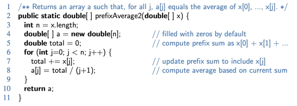
Prefix average algorithm 2
An intermediate value in the computation of the prefix average is the prefix sum $x_0 + x_1 + \cdots + x_j$. If we denote the prefix sum for the $j$th element as total, then the prefix average $a_j$ can be comptued as a[j] = total/(j+1). For greater efficiency as compared to the first algorithm, we can maintain the current prefix sum dynamically. This way, we only need one for loop.
Book’s implementation of algorithm 2
Experimental analysis of both algorithms’ runtime
Once you have both algorithms implemented, perform an experimental analysis of their runtimes. In a main method, implement tests for both of the prefix average algorithms with arrays filled with random values between 0 and 99. Show running time in nano seconds for input size of 10, 100, 1000, 10,000, and 100,000. Output the results, and a print statement with your estimate of asymptotic running time (constant, logarithmic, linear, n-log-n, quadratic, cubic, or exponential) based on the results of your experiments.
To fill the arrays of random values, use the nextDouble(double bound) method from java.util.Random.
Here are some ideas to help with estimating the asymptotic running time.
- Plot your runtimes with $n$ on the x-axis and the runtime on the y-axis.
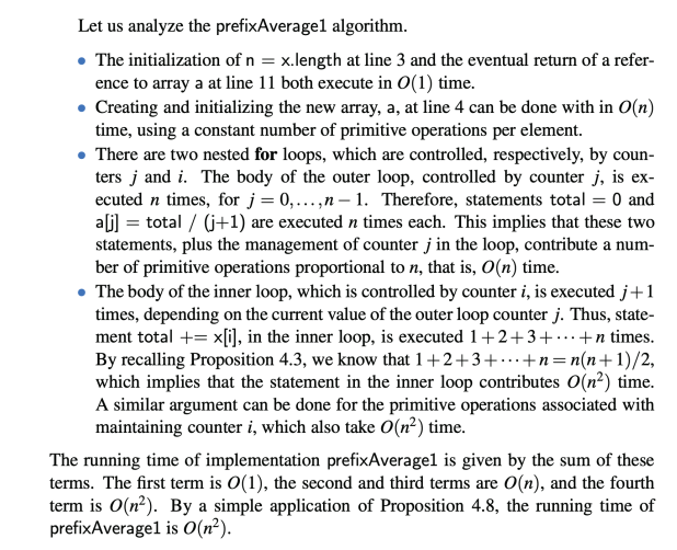
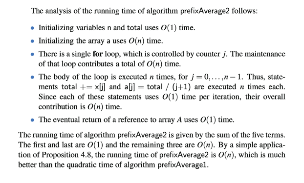
- For each algorithm, write down the number of primitive operations. What is the dominant term in each? The book has an example of this (don’t look if you want to try to do it on your own). Here is the analysis for algorithm 1 and here is the analysis for algorithm 2.
Sample output
The blanks should be filled in by your program.
n = 10    alg1 time: ___ ns.
n = 100    alg1 time: ___ ns.
n = 1000    alg1 time: ___ ns.
n = 10000    alg1 time: ___ ns.
n = 100000    alg1 time: ___ ns.

n = 10    alg2 time: ___ ns.
n = 100    alg2 time: ___ ns.
n = 1000    alg2 time: ___ ns.
n = 10000    alg2 time: ___ ns.
n = 100000    alg2 time: ___ ns.

These results indicate the growth function of first algorithm is ___ and second algorithm is ___.
Grading - 10 points
- 4 points - five tests of the first algorithm (with n equal to 10, 100, 1000, 10,000, and 100,000), and time in nanoseconds for each. Make sure that you are just timing the execution of the algorithm, not the creation of the random arrays. -1 point if you do that.
- 4 points - five tests of the second algorithm (with n equal to 10, 100, 1000, 10,000, and 100,000), and time in nanoseconds for each. Make sure that you are just timing the execution of the algorithm, not the creation of the random arrays. -1 point if you do that.
- 2 points - Your answers for running time of both algorithms.
Grading turnaround
This lab will be graded with scores in Brightspace before Tuesday, October 25th.
Go beyond
- Show that your theoretical analyses are correct by writing out the number of steps each algorithm takes as a function of the input size and showing that that function is Big-O of your claimed runtime. That is, give a $c$ and a $n_0$ that support your claim.